

How to use XLOOKUP in Excel is one of the first things you should learn if you’re tired of scrolling through rows and matching data manually.
“Why do I have to scroll and match things manually every time?”
Yeah, that gets old fast.
If you’ve ever tried to match names, IDs, or prices across columns, you know how messy it can get.
Here’s the good news:
XLOOKUP lets you find and return data instantly with one formula.
Let’s break it down step by step.
XLOOKUP Formula in Excel
The basic XLOOKUP formula is:
=XLOOKUP(lookup_value, lookup_array, return_array)
Here’s what each part means:
- lookup_value = the value you want to find
- lookup_array = the range where Excel looks for that value
- return_array = the range Excel pulls the result from
The commas are important because they separate each part of the formula. In other words, each comma tells Excel where one argument ends and the next one begins.
Key Takeaways
- XLOOKUP replaces manual matching by letting you find and return data instantly with a single formula
- The formula works using three main parts: lookup value, lookup array, and return array
- You don’t need complicated formulas anymore. XLOOKUP is simpler and more flexible than older functions like VLOOKUP
- Always lock your ranges using F4 before dragging the formula, or your results will break
- XLOOKUP can pull data from another sheet without any extra setup, which makes it useful for real-world messy data
- You can handle missing values easily by adding a fallback like “Not Found” instead of errors
- It works both vertically and horizontally, so you’re not limited to one data layout
- Once set up, the formula updates automatically when your data changes, saving time on repeated work
How to build & use an XLOOKUP formula in Excel
Steps:
- Select the cell where you want the result
- Start the XLOOKUP formula
- Select the lookup value
- Select the lookup array
- Select the return array
- Set optional parameters (if needed)
- Press Enter and apply the formula
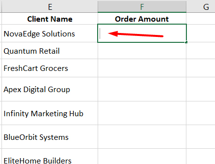
Step 1: Select the cell where you want the result
Click on the cell where you want Excel to return the matched value. This is where your result will appear after the formula runs.
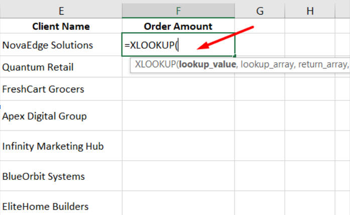
Step 2: Start the XLOOKUP formula
Type = and then type XLOOKUP(
Excel will show a small helper box with all the arguments you need to fill. Don’t worry about memorizing them yet. You’ll get used to it after a few uses.
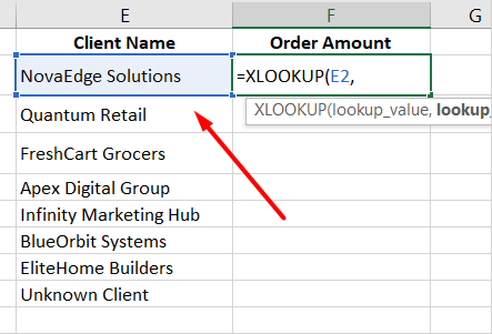
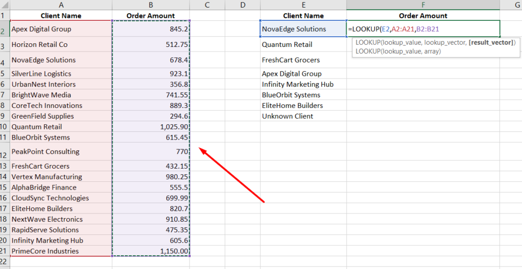
Step 3: Select the lookup value
Now click the cell that contains the value you want to search for. For example, if you’re trying to find a client’s order amount, click the cell with the client name, such as E2.
This is what Excel will try to match.
After selecting that cell, type a comma (,) to move to the next part of the XLOOKUP formula. Your formula should now look like this:
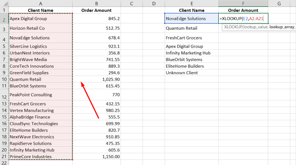
Step 4: Select the lookup array
Next, select the column or range where Excel should look for that value.
This is your “search area”.
If your client names are in column A, select that entire column or range. Then type a comma (,) to move to the next part.
Step 5: Select the return array
Now select the column that contains the result you want. If you want order amounts, select the column where those amounts exist.
So basically:
- Lookup array = where to search
- Return array = what to bring back
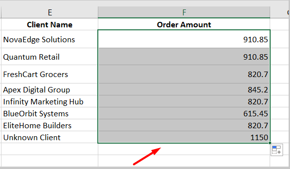
Step 6: Press Enter and apply the formula
Close the bracket ) and press Enter.
You’ll get your result instantly.
To apply it to other rows:
- Double-click the small square at the bottom-right of the cell
- Or drag it down
One important thing here…
Before dragging, lock your ranges using F4.
Otherwise, Excel will shift your ranges and break your formula.
📖 You May Also Like This “MS Excel” Article: How to Convert a Word Document to Excel
How to use XLOOKUP in Excel with two sheets
You’re not always working in one sheet. Real data is messy.
Sometimes your lookup data is in another sheet. XLOOKUP handles that easily.
Steps:
- Start the XLOOKUP formula in your current sheet
- Select the lookup value
- Switch to the second sheet
- Select the lookup array
- Select the return array
- Lock the ranges and press Enter
Step 1: Start the formula
Go to your working sheet and type:
=XLOOKUP(
Step 2: Select the lookup value
Click the value you want to search for (like a product name or client name).
Step 3: Switch to the second sheet
Now, click the sheet tab where your data exists.
Your formula bar will still stay active.
Step 4: Select the lookup array
Select the column that contains the matching values.
For example, all client names.
Step 5: Select the return array
Now select the column that contains the result you want.
For example, prices or order values.
Step 6: Lock the ranges and press Enter
Press F4 on both arrays to lock them.
Close the bracket and press Enter.
Now drag the formula across or down as needed.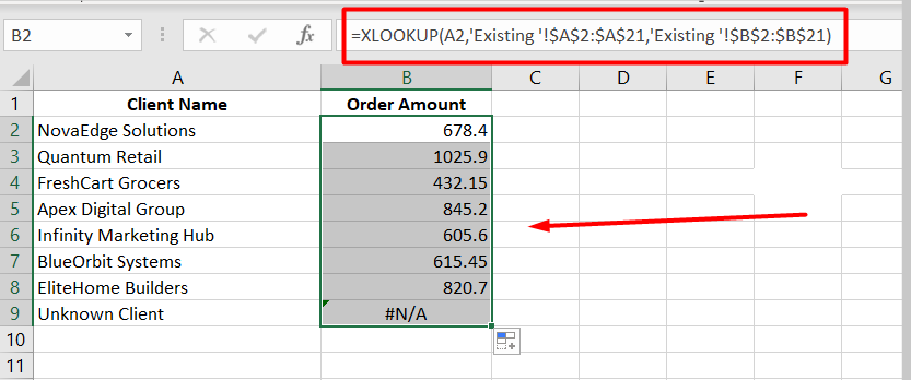
What does XLOOKUP do in Excel?
XLOOKUP searches for a value in one place and returns a related value from another place.
Simple example:
- Find a name
- Return the salary
Instead of manually scanning rows, Excel does it instantly.
It works both vertically and horizontally, which older functions struggled with.
📖 You May Also Like This “MS Excel” Article: How to Create a Clustered Column Chart in Excel
How does XLOOKUP work in Excel?
Think of XLOOKUP like this:
You give Excel 3 main things:
- What to search
- Where to search
- What to return
Excel goes through the lookup array, finds a match, and pulls the value from the return array.
If it doesn’t find anything, it can return a custom value like “Not Found”.
It’s dynamic too. If your data changes, results update automatically.
Where is the XLOOKUP function in Excel?
You won’t find XLOOKUP as a button.
It’s a formula.
Just type =XLOOKUP( in any cell, and Excel will show you the function helper.
If you want help while building it:
- Click the fx icon next to the formula bar
- It opens a guide with all arguments explained
FAQs
When was XLOOKUP added to Excel?
XLOOKUP was introduced with Microsoft 365 and later added to Excel 2021. It’s part of the newer generation of Excel functions.
What version of Excel has XLOOKUP?
XLOOKUP works in:
- Excel for Microsoft 365
- Excel 2021 and newer
Older versions like Excel 2016 or 2019 don’t support it.
Why does my Excel not have XLOOKUP?
Most likely, you’re using an older version of Excel.
If XLOOKUP doesn’t show up:
- Check your Excel version
- Update to Microsoft 365 or Excel 2021
Without that, the function simply won’t be available.